Framework for Automating HIL Tests

Version 1 of this project was presented at the MathWorks Automotive Conference in 2025

As a Controls Modeling and Analysis Lead Engineer at Nikola, I was responsible for controls validation using hardware-in-the-loop (HIL). HIL testing, as I inherited it, was inefficient—both in test authoring and execution. The project discussed below made the process more efficient.

Tech Stack

#

• Version 1:
  • MATLAB 2024a
• Version 2:
  • Python 3.10
  • Libraries:
    • Data wrangling and analysis: NumPy, Pandas
    • Excel writing: OpenPyXL
    • MATLAB interaction: matlabengine
    • Other: Internally built libraries (discussed later)

Background

#

Vehicles are equipped with electronic control units (ECUs) to control their functions. These units, or microcontrollers, control different systems in vehicles, including the body, frame, thermal, components, etc. In some architectures, each system or component may have its ECU. ECUs communicate with each other directly or through proxies to maintain smooth vehicle operation.

Like a personal computer, ECUs have inputs and outputs. Just as a keystroke produces a letter on the computer screen, an ECU input produces a certain output determined by its control logic. The interplay of all the vehicle’s control units shapes its operation. These involve simple behaviors like turning on cabin lights when a door opens or complex ones where airbags inflate during a crash. Hence, thorough testing of all units individually and as a system is paramount for a vehicle’s safety, reliability, and efficiency, and HIL allows us to do just that without being in an actual vehicle.

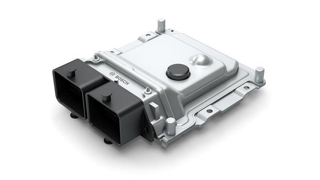
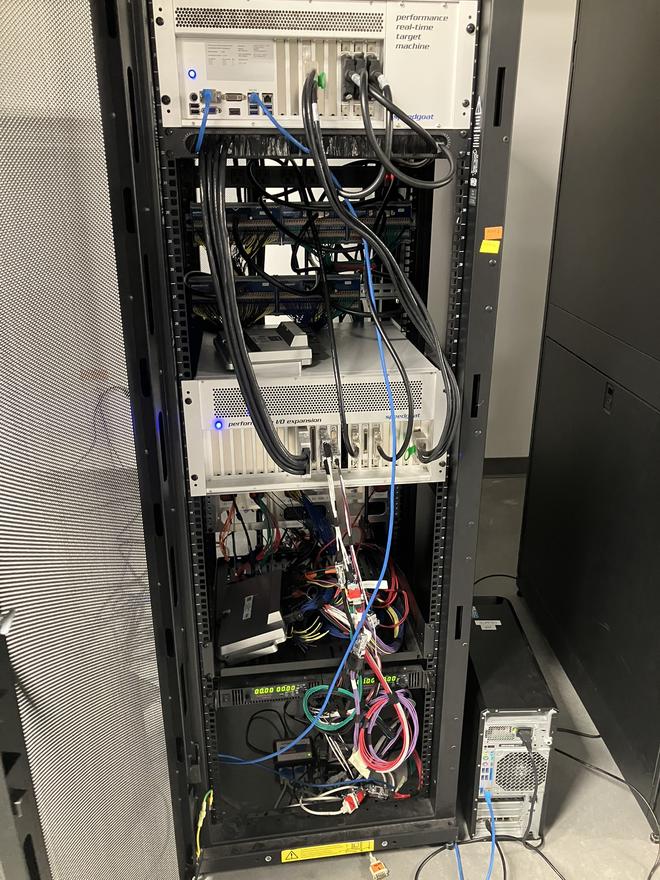
HIL isolates an ECU or a network of them, physically, for controls validation. A real-time computer probes the ECU with inputs and records its output, which is subsequently used to validate acceptable behavior. Systems models are used to mock the rest of the vehicle so that the ECU under test works without fault, similar to spoofing or mocking. These models, along with the test recipe, are uploaded to the real-time computer, which maintains its umbilical connection to the ECU via wire harnesses.

Old Process

#

Nikola’s HILs were made by Speedgoat, which had corporate ties with MathWorks. Therefore, only MathWorks tooling could be used to interact with the HIL. Specifically, the Simulink Test toolbox became the foundation for HIL testing, and Simulink the default option for creating system and test models. The flowchart sums up the process.

flowchart LR;
A[Test Model]-->|Provide inputs|B[Main Model];
B-->|Stimulates via real-time machine|C[ECU under test]

Main Model

#

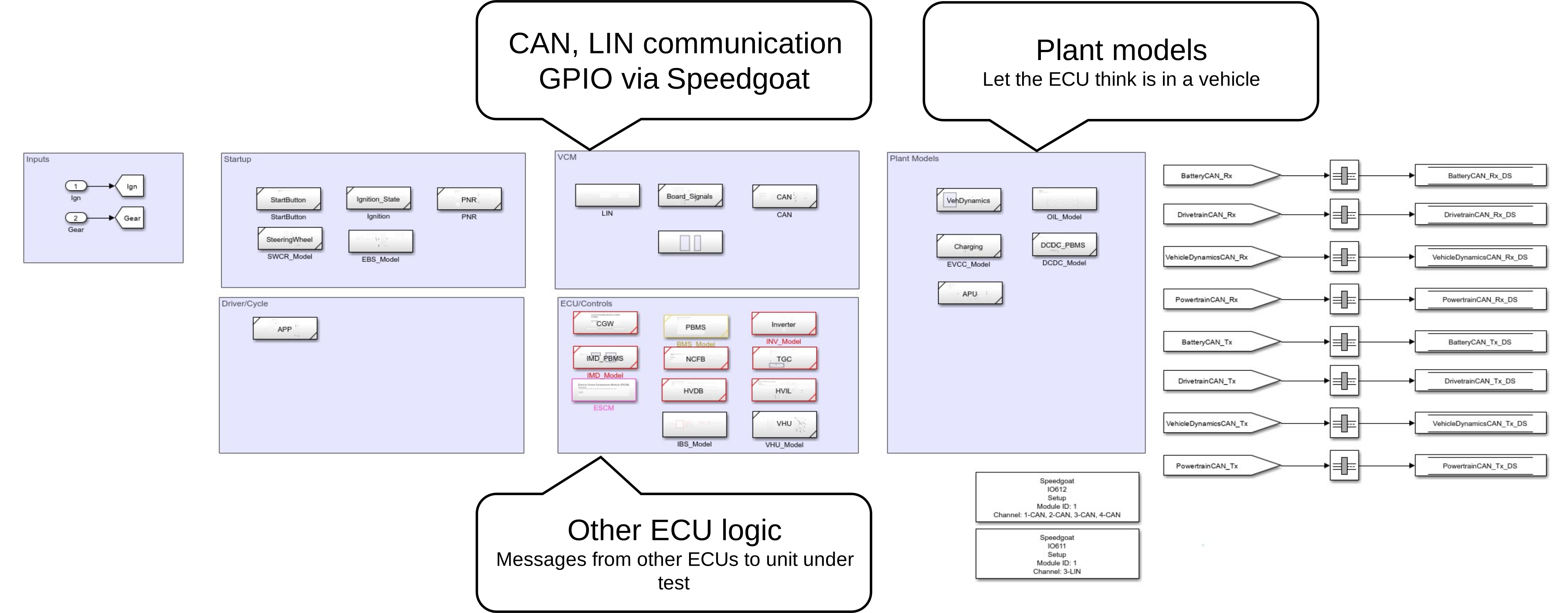
It all started with a main model with system models (or plant models), communication to and from the ECU under test (GPIO, CAN, and LIN), and other ECU logic that interacted with the unit under test. The model was a scaffolding for the ECU under test and mocked systems that the ECU relied on. For example, the vehicle control unit’s main model is shown below. Powertrain, battery, vehicle dynamics (kinematics) formed the system models that closed the loop with the ECU under test by applying first-principles logic to messages received from the ECU.

Test Model

#

The test model was a wrapper around the main model that included a sequence block for stepping through the test and an assessment block to verify signals in real time. This model probed the main model and was responsible for other HIL controls like power supply control for the ECU under test.

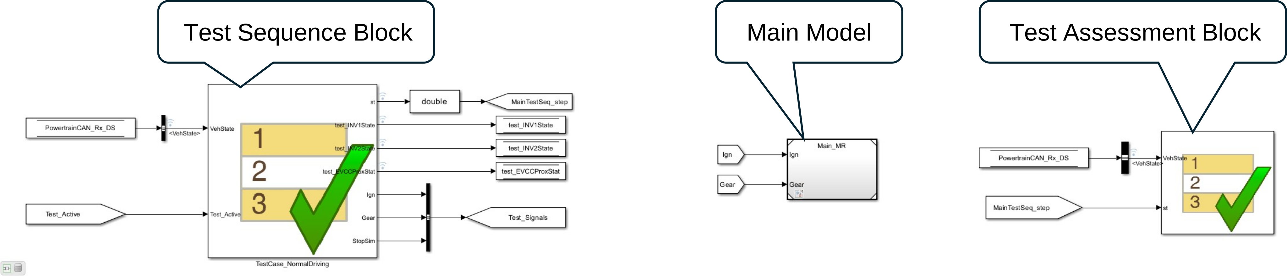
Individual test models represented separate tests. For example, there were 40 test models for the vehicle control unit.

Build and Test

#

All test models had to be compiled before test execution. Compilation was a three-step process, and for the vehicle control unit, it took 18-20 minutes for one test build. For 40 tests, that translated to approximately 12 hours of total build time. Test execution had its issues either from Test Manager or Speedgoat HIL initialization or other inexplicable crashes. Finally, it took about 4 days to run a regression of 40 tests—inadequate and inefficient.

flowchart LR;
A[Simulink Test Model]-->|Conversion|B[C code];
B-->|Compilation|C[Executable for HIL]

Disadvantages

#

The old process came with various disadvantages not just for test execution but also for test authoring.

1. Long Build Times

#

Long wait times not only caused delays from thought to execution but also friction in developing new tests, that led to poor test coverage. Build times were directly proportional to the complexity of the system model, and unlike the vehicle control unit’s model, others took only 8-10 minutes to compile.

2. Difficult Trial and Error

#

Long build times made trial and error difficult, where an engineer tries signal values beyond the requirement’s thresholds to incite a failure—a proven method to validate edge cases. It was responsible for poor test coverage in an existing test.

3. Lack of Reusability

#

During operation, ECUs change states along different logic lines based on input. For the vehicle control unit, it meant transitioning from Standby to HVOn to Drive. Most tests depended on the ECU being in a certain state, and the steps to achieve that state had to be repeated within every test model. There was no easy way to reuse these sequences without copying them in new tests, and it violated D.R.Y.

4. Lack of Maintainability

#

As various tests had the same logic to achieve a certain ECU test, a change in that logic meant updating it in all the affected test cases. The friction of this process left many tests without updated logic, and they languished as “old” tests, never to be used again. This further led to poor test coverage.

5. Message rates skewed

#

ECUs transmitted messages at different rates depending on the message information: 1 ms, 250 ms, 1 s, or 10 s intervals. The test model was tuned to 1 ms and interpolated all incoming ECU messages to that interval due to the real-time nature of the assessments. This led to incorrect validation.

I discovered this issue when validating a counter message with discrete 0 to 15 (an unsigned integer) transmitted every 500 ms. The model interpolation introduced floating-point values for this message before assertion in the assessment block and led to intermittent validation failures.

6. Missing robustness

#

Multiple intermittent failures plagued the validation procedure, and keeping track of these for each edge case became unwieldy. The non-repeatable nature made it difficult to find a robust solution for these failures.

Version 1

#

My goal was to eliminate these disadvantages and have a framework that made test authoring easier, and executed tests with log analysis and report generation with one command. And to do so expeditiously. Long build times were the opposite of expeditious.

slrealtime

#

Simulink Test ships with the slrealtime, which I learned about while presenting at the MathWorks Automotive Conference 2024. We made a graphical user interface for running HIL simulations, and that used slrealtime generously.

slrealtime is a quasi ASAM XIL abstraction of MATLAB. ASAM XIL is an API protocol to communicate between computers and test benches. It allows us to modify, read, and monitor the real-time machine’s state from a remote computer. slrealtime lets us initiate the real-time machine using tg = slrealtime('TargetPC1') and perform operations on the tg object:

tg.load('ModelName');                   % Loads model on target
tg.addInstrumentation(hInst);           % Adds instrumentation to read signals
tg.start('Stimulation', 'on');          % Starts the real-time machine with a model
tg.stop();                              % Stops the real-time machine/simulation
tg.getsignal('/path/to/block', 1);      % Gets signals using the added instrumentation
tg.setparam('', 'myParam', uint(42));   % Sets parameters while the simulation is running

As slrealtime could change parameters in the model by providing its full path, there was no need for a test sequence block. Separate test sequence blocks were responsible for separate test models that required individual builds. With that eliminated, I could use just one test model, reducing wait to merely 18-20 minutes. This model had all the controls and hooks needed to incite the desired behavior from the model, and adding a new hook meant only one build.

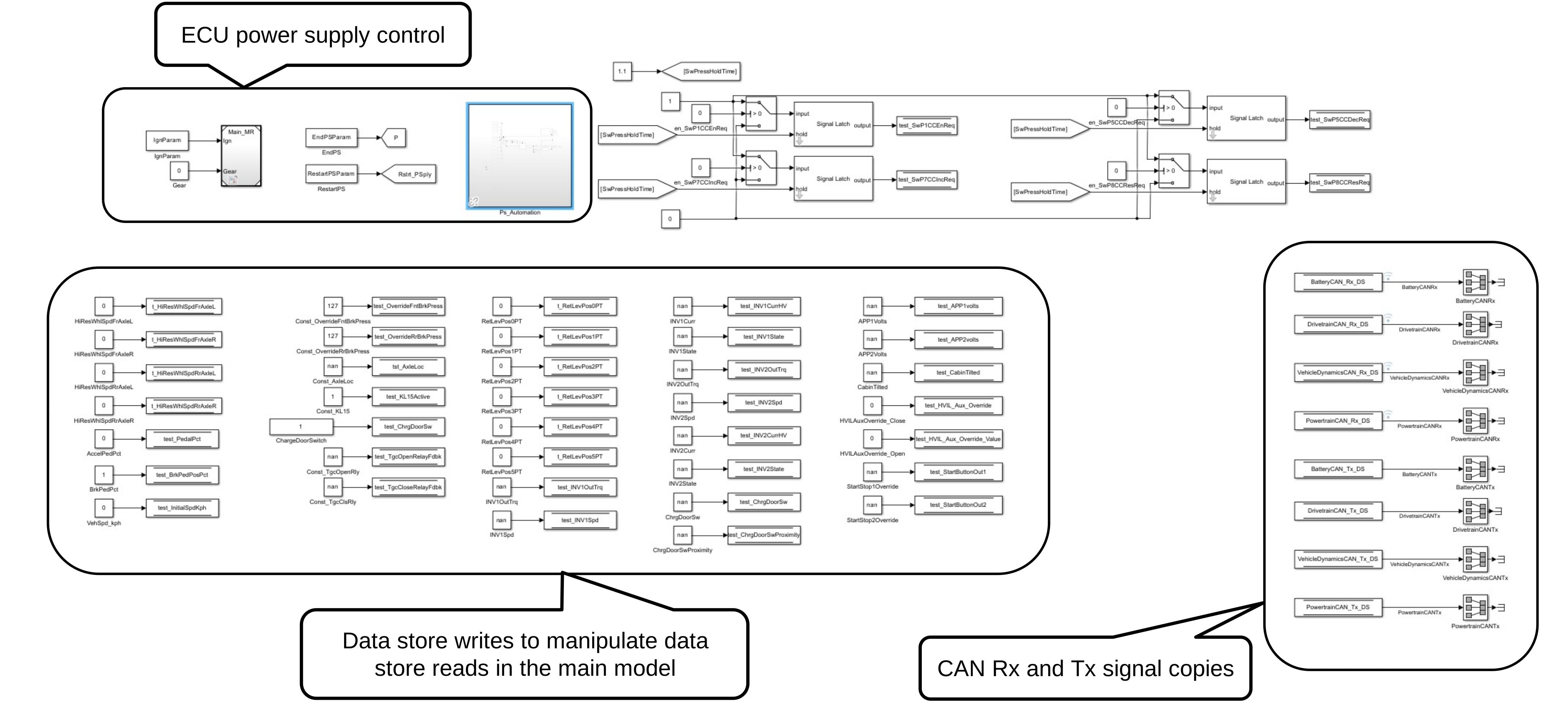
Reusable functions

#

One test could be abstracted as a sequential system with discrete steps. Most steps, however, were repeated for all tests, such as starting the test bench, loading models onto it, starting and stopping loggers, and cleanup. The actual steps were a small portion limited to setting up preconditions and running the test. Moreover, preconditions were repeatable behaviors to get the ECU in a particular state before running test steps. Therefore, such repeated steps (getVCMInxxx.m files) and preconditions (initiatexxxTests.m files) were abstracted out into reusable functions. The Appendix shows three such reusable functions.

flowchart TD;
A[Load model on target]-->B[Set pre-conditions];
B-->C[Start real-time machine]
C-->|Start data logger|D[Execute test logic]
D-->|Stop data logger|E[Clean up]
E-->F[Stop Target]

The functions eliminated two disadvantages: lack of reusability and maintainability. Being text files helped easy comparison and version control with tools like git diff. Lastly, if controls changed, only functions would need updates for the changes to be reflected in all tests.

├── changeVehSpd.m
├── closeCanalyzer.m
├── deactivateHVIL_AuxContactors_Overrides.m
├── disableBMSDiagEventStat.m
├── ESCOverrides.m
├── forceHVIL_AuxContactors.m
├── getACCTimeGapMode.m
├── getVCMInACC.m
├── getVCMInCharge.m
├── getVCMInDrive.m
├── getVCMInHVOn.m
├── getVCMInStandby.m
├── initiateACCTests.m
├── initiateDCDCSigs.m
├── initiateIMDStatSigs.m
├── initiateTest.m
├── killECUPowerAndStopTg.m
├── loadModelOnTargetPC.m
├── MBD_Cycle.m
├── openCanalyzer.m
├── overrideBattLinkVolt.m
├── overrideBattStrVolt.m
├── overrideFaultBMSHVIL.m
├── overrideBMSDemClntFlood.m
├── overrideBMSMax_Min_ModTemp.m
├── overrideBMSModTempStr.m
├── overrideBMSPrechrgState.m
├── overrideBMSStrState.m
├── pressCCButton.m
├── readValOnTarget.m
├── restartPowerSupply.m
├── runFaultClearUDSRoutine.m
├── separateBLFDataWithCAN.m
├── setHILMainTestSeq.m
├── setInvTrq.m
├── setBMSDemClntFlood.m
├── setBMSEmergReqFault.m
├── setBMSThermalFaultStat.m
├── setRegenLevel.m
├── setVehSpd.m
├── shiftVCMToPark.m
├── switchOffAndEndSim.m

Test Function

#

Reusable functions created the building blocks for writing effective tests. The test function itself used these methodically and added relevant test logic. The example below starts by using initateTest to load the model and start the HIL bench. If the HIL bench fails to start, the targetPC.isRunning checks for it and stops the test. Using another reusable function—getVCMInHVOn—the ECU is brought to the right state before the test steps. If the ECU does not reach that state in 50 seconds, the test would quit. Lines containing the pauses are the test steps. Finally, killECUPowerAndStopTg shuts the ECU down and the real-time machine.

function filename = tst_IMDStat_ExcitePulseOff()

    modelName = 'test_model';
    harnessName = 'tst_IMDStat_ExcitePulseOff';
    
    % Initiate test
    [targetPC, filename] = initiateTest(modelName, 1, harnessName);

    % Check if real-time machine started without issues. If not, clean up
    if ~targetPC.isRunning
        closeCanalyzer(false);
        return;
    end

    % Check if the ECU achieves HVOn state in 50 seconds. If it doesn't 
    % something is wrong. Clean up and return
    tic;
    while ~getVCMInHVOn(targetPC, modelName)
        if toc >= 50
            killECUPowerAndStopTg(targetPC);
            closeCanalyzer(false);
            return;
        end
        continue;
    end

    pause(30);
    targetPC.setparam('', 'PowertrainCAN_IMDStat_IMDExcitePulseOff',...
        TrueFalse_t.TrueFalse_True);
    pause(60);

    % Switch to park and turn the vehicle off
    killECUPowerAndStopTg(targetPC);
    closeCanalyzer(false);
    
    % Assessment calls
    testDets = assessResults(filename);
end

function assessResults()
% Rest of the assessment
end

Assessments

#

slrealtime when combined with tg.addInstrumentation dumped all the data as a logsout variable in the global MATLAB workspace. This was used to assess individual messages and determine pass/fail. The assessResults function below uses evalin to consume the global logsout variable into its local workspace. It finds variables in logsout to obtain specific messages—VehState and VCMDiag—for extracting relevant information at particular timestamps. A typical assessResults function returned an Excel row with relevant columns to be part of the report.

With test and assessment functions, trial and error was easier, and the time it took from thought to execution reduced drastically.

function testDets = assessResults(faultLvl, filename)
% Function assesses results for the fault management test cases based on
% the faultLvl that is sent to the caller

    logsout = evalin('base', 'logsout');
    powCANRx = logsout.find('PowertrainCANRx');
    vcmFaultLvl = powCANRx.Values.VCMDiag.VCMFaultLvl;
    vehState = powCANRx.Values.VehState.VehState;
    desFaultLvlTm = vcmFaultLvl.Time(vcmFaultLvl.Data == faultLvl);

    testDets = {filename, 'Fault management', 'Req-Num-00000', ...
        ['Set fault level to ' char(faultLvl)]};
    ... % rest of the assessment
end

logsout, as the test assessment block before, was still susceptible to interpolating messages to match the model’s 1 ms interval rate. This disadvantage was resolved only in Version 2.

Framework

#

With the strong base of test and assessment functions, I created a framework to run regression tests using one command. This framework used MATLAB’s unittest object-oriented programming interface, similar to Python’s standard library unit test framework, to set up, tear down, and run tests. An example test class highlights the details of this framework. The resultsTable property, accessible from all class methods, receives a header in the setup and is updated with each test method’s results. During the tear down, resultsTable is converted to an Excel file using writetable. After each test, in the test method tear down, logsout is cleared from the base workspace to free up RAM.

classdef BMSVCMValidation < matlab.unittest.TestCase

    properties
        resultsTable;
    end

    methods(TestClassSetup)
        % Shared setup for the entire test class
        function setUp(tc)
        % Sets up a table for writing data and 
           tableHeader = {'Filename', 'Fault Response', 'Test Type', ...
            'Drive Scenario', 'Expectation', 'Actual', ...
            'Result'};
            rt = cell2table(cell(0, 7), 'VariableNames', ...
                tableHeader);

            tc.resultsTable = rt;
        end
    end

    methods(TestClassTeardown)
        % Shared teardown for the entire test class
        function saveExcel(tc)
            dtNow = string(datetime, 'yyyy-MM-dd_hh-mm-ss');
            writetable(tc.resultsTable, ['Results/BMSVCMValidation_' char(dtNow) '.xlsx']);
        end
    end

    methods(TestMethodSetup)
        % Setup for each test
    end

    methods(TestMethodTeardown)
        % Teardown for each test
        function tearDownEach(tc)
            writetable(tc.resultsTable, tc.excelFile, 'WriteMode', 'append');
            tc.resultsTable = tc.emptyResultsTable;
            
            % Clear logsout
            evalin('base', 'clear logsOut;');
            Simulink.sdi.clear;
        end
    end

    methods(Test)
        % Test methods
        function tst_HVStrVoltDelta_tc(tc)
        % Tests HVStrVolt delta for various scenarios and adds the results
        % to a table for excel outputting
            voltDiff = 12.1;
            numOfPacks = 1;
            testDets = tst_HVStrVoltDelta(numOfPacks, voltDiff);
            tc.resultsTable = [tc.resultsTable; testDets];
        end

        ... % rest of the tests
    end
end

Multiple control pathways

#

Classes were created for validating each control logic pathway for maximum test coverage.

├── BMSInit
├── CruiseControl
├── Cybersecurity
├── OneOffs
├── BMSVCMValidation
├── TorqueMonitoring
├── VF1_VehicleState
├── VF2_TorqueCommand
├── VF9_Fault_Management
├── VF12_ThermalIndicators
└── VPE_Req

To run the entire regression suite, I created a runRegression function that leveraged MATLAB’s built-in runtests (part of the matlab.unittest.TestCase API). Thus, one command—runRegression()—ran all the tests, assessed results, and generated a report.

function runRegression()
% Runs the entire regression suite with all the logical pathways

    logicPaths = { ...
        'BMSInit', ...
        'CruiseControl', ...
        % rest of the classes
    }

    % Run tests using MATLAB's built-in runtests
    cellfun(@(logicPath) runtests(logicPath), logicPaths)
end

Impact (so far)

#

With the new framework and a few weeks, I had written 462 tests for the vehicle control unit, up from 40 tests, i.e., a 10-fold increase in test coverage. The process development was underscored by a critical safety recall of the BEV trucks and helped extend this framework to add validation for a battery supplier change.

Problems

#

Fissures in the process started to emerge. A complete regression could not be completed due to excessive RAM usage of MATLAB. The main cause was logsout which represented all the data downloaded from the HIL bench. Pictures below show a progression of RAM usage until the OS had to stop the MATLAB session after approximately 15 tests.

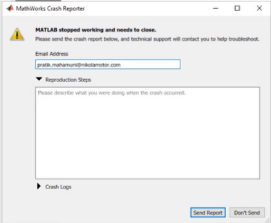
Even by implementing multiple solutions to return RAM back to the OS, memory consumption still stayed high, and regression tests never completed.

% Things I tried to release RAM back to the OS

% 1. Clear logsout after analysis is complete
evalin('base', 'clear logsout;')

% 2. Clear Simulink cache
Simulink.sdi.clear;

% 3. Invoke JAVA garbage collection
java.lang.System.gc();
java.lang.Runtime.getRuntime().gc;

Version 2

#

I turned to Python for creating an orchestrator to manage MATLAB sessions, a wrapper around the test framework that handled errors gracefully and created a truly automated system. The orchestrator also allowed certain redundancy checks and retry logic that added robustness to the framework.

Python and matlabengine

#

Python, with its rich library support, had matlabengine, a library created by MathWorks themselves for interacting with MATLAB sessions. The library allows opening MATLAB sessions in the background (with the -nodesktop flag) and running commands in that session using Python. start_matlab_project shown below did just that and returned the handle to the MATLAB session.

A non-trivial MATLAB project, with numerous imports or global variables, can be saved as a MATLAB Project (.prj file). The .prj file stores this information and adds these to the global workspace on initiation. Large projects can take up to 5 minutes to load in a given MATLAB session.

import matlab.engine

def start_matlab_project():
    """
    Starts MATLAB and the project that is relevant to the folder / directory
    we are in
    """
    engine = matlab.engine.start_matlab("-nodesktop")
    engine.openProject("../..")  # type: ignore

    return engine

Retry logic, shown below, guarded against intermittent failures such as MATLAB crashes, HIL bench start-up issues, ECU state not ready for tests, and even logger failures. It tried any test thrice before moving on, ensuring that other regression tests would complete without stopping. With robust logs, it was easy to pinpoint failed tests and rerun them manually.

def retry_if_failed(
    matlab_eng, test_func: Callable, des_vehstate: int, *args, **kwargs
) -> Tuple[bool, str]:
    retries = 0
    veh_state_ach = False

    blf_filename: str = ""
    while not veh_state_ach:
		if retries > 3:
            return False, blf_filename
        
        try:
            blf_filename = test_func(*args, **kwargs)
            cast(str, blf_filename)
            veh_state_ach = is_vehstate_achieved(blf_filename, des_vehstate)
        except:
            matlab_eng.closeCanalyzer(False)

        retries += 1

    return True, blf_filename

Handshake

#

As shown before, fifteen tests led to MATLAB’s crash. I developed a way to run ten tests in any MATLAB instance, close it, and continue the next set of 10 tests into a new instance. For consistency with the MATLAB-only framework (discussed here), I had created a Python class for each control logic pathway used to execute and analyze tests. This class had two properties defined in the __init__() method:

class BMSVCMValidation:
    def __init__(self):
        self._current_mateng = None
        self._new_mateng = None
        # rest of the class

Before the first test, self._current_mateng would be initiated:

self._current_mateng = start_matlab_project()
self.run_hv_strvolt_delta()
# Rest of the tests

And after ten tests, that instance would be destroyed and replaced by a new instance:

self._current_mateng.quit()  # type: ignore
self._current_mateng = start_matlab_project()
# Begin next set of tests

This logic worked for “standalone” tests. For batch tests run in a for loop to validate multiple battery packs of our nine-battery pack truck, a new MATLAB instance was opened after the seventh test. This ensured that the new session had enough time to fully load the .prj file. A “handshake” happened between self._current_mateng and self._new_mateng after the full for loop had finished execution; see the flowchart below.

flowchart TB
    subgraph NM[New MATLAB Instance]
    A1["Test 1"]-->C1["..."]-->D1["Test 7"]-->E1["..."]-->F1["Test 10"]
    end
    subgraph CM[Current MATLAB Instance]
    A["Test 1"]-->C["..."]-->D["Test 7"]-->E["..."]-->F["Test 10"]
    end
    D --Start new after 7th test--> NM
    F --Next test on new--> A1

def run_thermal_fault_stat_in_acc(self):
    for i in range(9):
        blf_filename, result = self._run_thermal_fault_stat(15, i)
        row = [
            blf_filename,
            # Other information of the test in this row
            "Pass" if result else "Fail",
        ]
        write_excel_row(self._results_path, [row])

        if i >= 7:
            self._new_mateng = start_matlab_project()

    self._current_mateng.quit()  # type: ignore
    self._current_mateng = self._new_mateng

Assessments

#

What I have not mentioned so far is that my HIL setup recorded ECU logs or vehicle logs using CANalyzer loggers for redundancy. This was key for not using logsout with its funky interpolations. I created a library to parse CAN and LIN data from ECU log files, use DBC files to extract relevant data, and perform assertions. I talk about that library here. The library’s API provided an important function, extract_messages, which extracted messages passed to it as a list. This library, along with the venerable NumPy and Pandas libraries, paved a path for assessment functions in Python.

retry_if_failed, shown above, calls one such assessment function: is_vehstate_achieved.

def is_vehstate_achieved(blf_filename: str, des_vehstate: int) -> bool:
    blf_filepath = Path(HIL_LOGS, f"{blf_filename}.BLF")
    dbc_files = [Path(TRE_COMMS_DIR, "/path/to/PowertrainCAN.dbc")]
    messages = ["VehState"]

    data = extract_messages(blf_filepath, dbc_files, messages)
    vehstate = data["VehState"]["VehState"].to_numpy()
    vehstate_filt = vehstate[vehstate == des_vehstate]

    if vehstate_filt.size == 0:
        return False
    else:
        return True

Impact

#

Version 2 catapulted HIL tests from being manual to running without human intervention. Most failures were handled gracefully, and regression tests were fully automated. My proof of concept on the vehicle control unit was now able to run 462 tests in under 20 hours. The framework was pip installable, which meant all HIL benches could benefit from these optimizations. Engineers were now free to develop new tests, and validate controls in novel ways.

Appendix

#

1. Loading the model on the target and setting up instrumentation

flowchart TD;
A[Load model on target]-->B[Set pre-conditions];
B-->C[...]

style A fill:#e879f9,stroke:#e879f9

function targetPC = loadModelOnTargetPC(modelName)
% Loads model on target pc
    
    arguments
        modelName char;
    end
    targetPC = slrealtime('TargetPC1');

    removeAllInstruments(targetPC);
    load(targetPC, modelName);

    hInst = slrealtime.Instrument(modelName);
    hInst.addSignal({'test_torquemonitoring/Data Store Read'}, 1); % BattCANRx
    
    % Add instrument object to target object
    addInstrument(targetPC, hInst);
end

2. Initiate Test

flowchart TD;
A[...]-->B[Set pre-conditions];
B-->C[Start real-time machine]
C-->|Start data logger|D[...]

style B fill:#e879f9,stroke:#e879f9
style C fill:#e879f9,stroke:#e879f9

• Setting pre-conditions before the ECU is powered on (setRegenLevel, targetPC.setparam)
• Starting the real-time computer (start(targetPC ...))
• Starting the logger for recording data (openCanalyzer)
• Starting the power supply to the ECU (restartPowerSupply)
• Setting more preconditions after the ECU is powered on (initiateDCDCSigs, initiateIMDStatSigs)

function [targetPC, filename] = initiateTest(modelName, regenLevel, harnessName, stopTime)
% Initiates the test by starting stimulation and restarting the
% power supply after some time.

    arguments
        modelName char;
        regenLevel single;
        harnessName char;
        stopTime double = 3600;
    end

    % Initiate test
    targetPC = loadModelOnTargetPC(modelName);
    filename = openCanalyzer(harnessName);

    % Start the simulation
    start(targetPC, 'StartStimulation', 'on', 'ExportToBaseWorkspace', true, ...
        'ReloadOnStop', false, 'StopTime', stopTime);

    pause(5);
    setRegenLevel(targetPC, modelName, regenLevel)
    targetPC.setparam([modelName '/BrkPedPct'], 'Value', 0);
    targetPC.setparam('', 'VehicleDynamicsCAN_StblCtrlStat_VDCFullyOp', ...
        ActvInactvSNA_t.ActvInactvSNA_Actv);
    
    % Start power supply
    restartPowerSupply(targetPC);

    % Initiate DCDC signals
    initiateDCDCSigs(targetPC);
    % Initiate IMD stat signals using the function that was created for it
    initiateIMDStatSigs(targetPC)
end

3. Clean up and stop real-time

It cleans up variables on the real-time target after the test (deactivateHIL_...), shuts the power supply for the ECU (targetPC.setparam('', 'EndPSParam', 1)), and finally stops the HIL bench (stop(targetPC)).

flowchart TD;
D[...]
D-->|Stop data logger|E[Clean up]
E-->F[Stop Target]

style E fill:#e879f9,stroke:#e879f9
style F fill:#e879f9,stroke:#e879f9

function killECUPowerAndStopTg(targetPC)
% Kills ECU power and stops the target computer

    arguments
        targetPC slrealtime.Target;
    end

    deactivateHVIL_AuxContactors_Overrides(targetPC);

    targetPC.setparam('', 'EndPSParam', 1);
    pause(1);
    stop(targetPC);
end